
The Global Temperature Jigsaw Explained
By Stefan Rahmstorf
18 December, 2013
Realclimate.org
Since 1998 the global temperature has risen more slowly than before. Given the many explanations for colder temperatures discussed in the media and scientific literature (La Niña, heat uptake of the oceans, arctic data gap, etc.) one could jokingly ask why no new ice age is here yet. This fails to recognize, however, that the various ingredients are small and not simply additive. Here is a small overview and attempt to explain how the different pieces of the puzzle fit together.
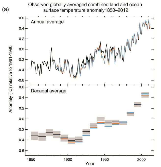
Figure 1 The global near-surface temperatures (annual values at the top, decadal means at the bottom) in the three standard data sets HadCRUT4 (black), NOAA (orange) and NASA GISS (light blue). Graph: IPCC 2013.
First an important point: the global temperature trend over only 15 years is neither robust nor predictive of longer-term climate trends. I’ve repeated this now for six years in various articles, as this is often misunderstood. The IPCC has again made this clear (Summary for Policy Makers p. 3):
Due to natural variability, trends based on short records are very sensitive to the beginning and end dates and do not in general reflect long-term climate trends.
You can see this for yourself by comparing the trend from mid-1997 to the trend from 1999 : the latter is more than twice as large: 0.07 instead of 0.03 degrees per decade (HadCRUT4 data).
Likewise for data uncertainty: the trends of HadCRUT and NASA data hardly differ in the long term, but they do over the last 15 years. And the small correction proposed recently by Cowtan & Way to compensate for the data gap in the Arctic almost does not change the HadCRUT4 long-term trend, but it changes that over the last 15 years by a factor of 2.5.
Therefore, it is a (by some deliberately promoted) misunderstanding to draw conclusions from such a short trend about future global warming, let alone climate policy. To illustrate this point, the following graph shows one simulation from the CMIP3 model ensemble:
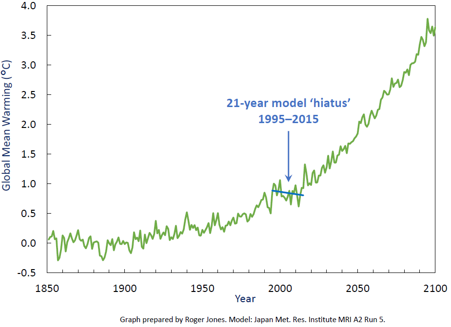
Figure 2 Temperature evolution in a model simulation with the MRI model. Other models also show comparable “hiatuses” due to natural climate variability. This is one of the standard simulations carried out within the framework of CMIP3 for the IPCC 2007 report. Graph: Roger Jones.
In this model calculation, there is a “warming pause” in the last 15 years, but in no way does this imply that further global warming is any less. The long-term warming and the short-term “pause” have nothing to do with each other, since they have very different causes. By the way this example refutes the popular “climate skeptics” claim that climate models cannot explain such a “hiatus” – more on that later.
Now for the causes of the lesser trend of the last 15 years. Climate change can have two types of causes: external forcing or internal variability in the climate system.
External forcing: the sun, volcanoes & co.
The possible external drivers include the shading of the sun by aerosol pollution of the atmosphere by volcanoes (Neely et al., 2013) or Chinese power plants (Kaufmann et al. 2011). Second, a reduction of the greenhouse effect of CFCs because these gases have been largely banned in the Montreal Protocol (Estrada et al., 2013). And third, the transition from solar maximum in the first half to a particularly deep and long solar minimum in the second half of the period – this is evidenced by measurements of solar activity, but can explain only part of the slowdown (about one third according to our correlation analysis).
It is likely that all these factors indeed contributed to a slowing of the warming, and they are also additive – according to the IPCC report (Section 9.4) about half of the slowdown can be explained by a slower increase in radiative forcing. A problem is that the data on the net radiative forcing are too imprecise to better quantify its contribution. Which in turn is due to the short period considered, in which the changes are so small that data uncertainties play a big role, unlike for the long-term climate trends.
The latest data and findings on climate forcings are not included in the climate model runs because of the long lead time for planning and executing such supercomputer simulations. Therefore, the current CMIP5 simulations run from 2005 in scenario mode (see Figure 6) rather than being driven by observed forcings. They are therefore driven e.g. with an average solar cycle and know nothing of the particularly deep and prolonged solar minimum 2005-2010.
Internal variability: El Niño, PDO & co.
The strongest internal variability in the climate system on this time scale is the change from El Niño to La Niña – a natural, stochastic “seesaw” in the tropical Pacific called ENSO (El Niño Southern Oscillation).
The fact that El Niño is important for our purposes can already be seen by how much the trend changes if you leave out 1998 (see above): El Niño years are particularly warm (see chart), and 1998 was the strongest El Niño year since records began. Further evidence of the crucial importance of El Niño is that after correcting the global temperature data for the effect of ENSO and solar cycles by a simple correlation analysis, you get a steady warming trend without any recent slowdown (see next graph and Foster and Rahmstorf 2011). ENSO is responsible for two thirds of the correction. And if you nudge a climate model in the tropical Pacific to follow the observed sequence of El Niño and La Niña (rather than generating such events itself in random order), then the model reproduces the observed global temperature evolution including the “hiatus” (Kosaka and Xie 2013) .
One can also ask how the observed warming fits the earlier predictions of the IPCC . The result looks like this (Rahmstorf et al 2011):
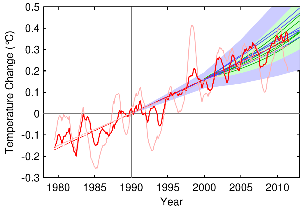
Figure 3 Comparison of global temperature (average over 5 data sets, including 2 satellite series) with the projections from the 3rd and 4 IPCC reports. Pink: the measured values. Red: data after adjusting for ENSO, volcanoes and solar activity by a multivariate correlation analysis. The data are shown as a moving average over 12 months. From Rahmstorf et al. 2012.
And what about the ocean heat storage ? That is no additional effect, but part of the mechanism by which El Niño years are warm and La Niña years are cold at the Earth’s surface. During El Niño the ocean releases heat, during La Niña it stores more heat. The often-cited data on the heat storage in the ocean are therefore just further evidence that El Niño plays a crucial role for the “pause”.
Leading U.S. climatologist Kevin Trenberth has studied this for twenty years and has just published a detailed explanatory article. Trenberth emphasizes the role of long-term variations of ENSO, called pacific-decadal oscillation (PDO). Put simply: phases with more El Niño and phases with predominant La Niña conditions (as we’ve had recently) may persist for up to two decades in the tropical Pacific. The latter brings a somewhat slower warming at the surface of our planet, because more heat is stored deeper in the ocean. A central point here: even if the surface temperature stagnates our planet continues to take up heat. The increasing greenhouse effect leads to a radiation imbalance: we absorb more heat from the sun than we emit back into space. 90% of this heat ends up in the ocean due to the high heat capacity of water. The fact that the ocean continues to heat up, without pause, demonstrates that the greenhouse effect has not subsided, as we have discussed here.
How important the effect of El Niño is will be revealed at the next decent El Niño event. I have already predicted last year that after the next El Niño a new record in global temperature will be reached again – a forecast that probably will be confirmed or falsified soon.
The Arctic data gap
Recently, Cowtan & Way have shown that recent warming was underestimated in the HadCRUT data. After using satellite data and a smart statistical method to fill gaps in the network of weather stations, the global warming trend since 1998 is 0.12 degrees per decade – that is only a quarter less than the long-term trend of 0.16 degrees per decade measured since 1980. Awareness of this data gap is not new – Simmons et al. have shown already in 2010 that global warming is underestimated in the HadCRUT data, and we have discussed the Arctic data hole repeatedly since 2008 at RealClimate. NASA GISS has always filled the data gaps by interpolation, albeit with a simpler method, and accordingly the GISTEMP data show hardly a slowdown of warming.
The spatial pattern
Cohen et al. have shown two years ago that it is mainly the recent cold winters in Eurasia that have contributed to the flattening of the global warming curve (see figure).
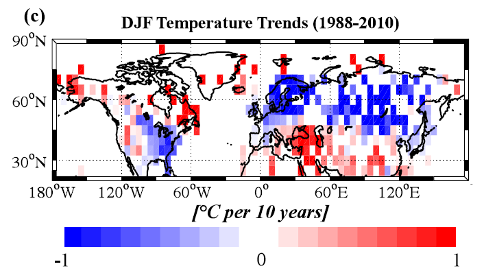
Figure 4 Observed temperature trends in the winter months. Despite the significant global warming in the annual mean, there was a winter cooling in Eurasia. CRUTem3 data (land only!), from Cohen et al. 2012.
They argue that an explanation for the “pause” in global warming would have to explain this particular pattern. But this is not compelling: there could be two independent mechanisms superimposed. One that dampens global warming – which would have to be explained by the global energy balance. And a second one that explains the cold Eurasian winters, but without affecting the global mean temperature. I think the latter is likely – these recent cold winters are part of the much-discussed “warm Arctic – cold continents” pattern (see, eg, Overland et al 2011) and could be related to the dwindling ice cover on the Arctic Ocean, as we explained here. Since the heat is just moved around, with Eurasian cold linked to a correspondingly warmer Arctic, this hardly affects the global mean temperature – unless you’re looking at a data set with a large data gap in the Arctic …
What does it add up to?
How does all that fit together now? As described above, I think (just like Trenberth) that natural variability, in particular ENSO and PDO, is the main reason the recent slower warming. From the perspective of the planetary energy balance heat storage in the ocean is the key mechanism.
If the warming is steady after adjusting for ENSO, volcanoes and solar cycles, does the additional correction for the Arctic data gap by Cowtan & Way mean that the warming after these adjustments has even accelerated? That could be, but only by a small amount. As you can see in Figure 6 of our paper (Foster and Rahmstorf), the slowdown is gone after said adjustment in the GISS data and the two satellites series, but there still is some slowdown in the two data sets with the Arctic gap, ie HadCRUT and NCDC. Adding the trend correction by 0.08 degrees per decade from Cowtan & Way to our ENSO-adjusted HadCRUT trend from 1998, you end up at about 0.2 degrees per decade, practically the same value as we got for the GISS data. If one further adds the effect of the above forcings (without the solar activity already accounted for) this would add a few hundredths of a degree. The result would be a bit faster warming than over the entire period since 1980, but probably less than the 0.29 °C per decade measured over 1992-2006. Nothing to get excited about. Especially since based on the model calculations you’d expect anyway trends around 0.2 degrees per decade, because models predict not a constant but a gradually accelerating warming. Which brings us to the comparison with models.
Comparison with models
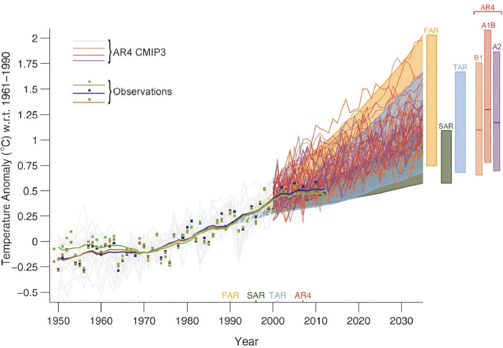
Figure 5 Comparison of the three measured data sets shown at the outset with earlier IPCC projections from the first (FAR), 2nd (SAR) 3rd (TAR) and 4th (AR4) IPCC report, as well as with the CMIP3 model ensemble. As you can see the data move within the projected ranges. Source: IPCC AR5, Figure 1.4. (Small note: “climate skeptics” brought an earlier, erroneous draft version of this graphic to the public, although it was marked in block letters as a temporary placeholder by IPCC.)
When comparing data with models, one needs to understand a key point: the models also produce internal variations, including ENSO, but as this (similar to the weather in the models) is a stochastic process, the El Niños and La Niñas are distributed randomly over the years. Therefore, only in rare cases a model will randomly produce a sequence that is similar to the observed sequence with reduced warming from 1998 to 2012. There are such models – see the first image above – but most show such phases of slow warming or “hiatus” at other times.
The IPCC has therefore never tried to predict the climate evolution over 15 years, because that’s just too much influenced by random internal variability (such as ENSO), which we cannot predict (at least as yet).
However, all models show such variability – no one who understands this issue could have been surprised that there can be such hiatus phases. They’ve also occurred in the past, for example from 1982, as Trenberth shows in his Figure 4.
The following graph shows a comparison of observational data with the CMIP5 ensemble of model experiments that have been made for the current IPCC report. The graph shows that the El Niño year 1998 is at the top and the last two cool La Niña years are at the bottom of the model projection range (for the various reasons explained above). However, the temperatures (at least according to the data of Cowtan & Way) are within the range which is spanned by 90% of the models.
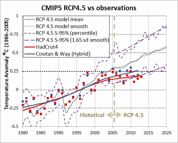
Figure 6 Comparison of 42 CMIP5 simulations with the observational data. The HadCRUT4 value for 2013 is provisional of course, still without November and December. (Source: DeepClimate.org)
So there is no evidence for model errors here (for more on this see this article) . This is also no evidence for a lower climate sensitivity, even if this was proposed some time ago by Otto et al. (2013). Trenberth et al. suggest that even the choice of a different data set of ocean heat content would have increased the climate sensitivity estimate of Otto et al. by 0.5 degrees. In addition, Otto et al. used the HadCRUT4 temperature data with its particularly low recent warming. With an honest appraisal of the full uncertainty, also in the forcing, one must come to the conclusion that such a short period is not sufficient to draw conclusions about the climate sensitivity.
Conclusion
Global temperature has in recent years increased more slowly than before, but this is within the normal natural variability that always exists, and also within the range of predictions by climate models – even despite some cool forcing factors such as the deep solar minimum not included in the models. There is therefore no reason to find the models faulty. There is also no reason to expect less warming in the future – in fact, perhaps rather the opposite as the climate system will catch up again due its natural oscillations, e.g. when the Pacific decadal oscillation swings back to its warm phase. Even now global temperatures are very high again – in the GISS data, with an anomaly of + 0.77 °C November was warmer than the previous record year of 2010 (+ 0.67 °), and it was the warmest November on record since 1880.
![]()
PS: This article was translated from the German original at RC’s sister blog KlimaLounge. KlimaLounge has been nominated as one of 20 blogs for the award of German science blog of the year 2013. If you’d like to vote for us: simply go to this link, select KlimaLounge in the list and press the “vote” button.
 Stefan Rahmstorf is a physicist and oceanographer by training, Stefan Rahmstorf has moved from early work in general relativity theory to working on climate issues. He has done research at the New Zealand Oceanographic Institute, at the Institute of Marine Science in Kiel and since 1996 at the Potsdam Institute for Climate Impact Research in Germany (in Potsdam near Berlin). His work focuses on the role of ocean currents in climate change, past and present. In 1999 Rahmstorf was awarded the $ 1 million Centennial Fellowship Award of the US-based James S. McDonnell foundation. Since 2000 he teaches physics of the oceans as a professor at Potsdam University. Rahmstorf is a member of the Advisory Council on Global Change of the German government and of the Academia Europaea. He is a lead author of the paleoclimate chapter of the 4th assessment report of the IPCC.
References
1. K. Cowtan, and RG Way, “Coverage bias in the HadCRUT4 temperature series and its impact on recent temperature trends”, Quarterly Journal of the Royal Meteorological Society, pp. n / an / a, 2013. http://dx.doi.org/10.1002/qj.2297
2. RR Neely, OB Toon, S. Solomon, J. Vernier, C. Alvarez, JM English, KH Rosenlof, MJ Mills, CG Bardeen, JS Daniel, and JP Thayer, ”
Recent Increases in anthropogenic SO2from Asia have minimal impact on stratospheric aerosol
“Geophysical Research Letters, vol. 40, pp. 999-1004, 2013. http://dx.doi.org/10.1002/grl.50263
3. RK Kaufmann, H. Kauppi, ML man, and JH Stock, “Reconciling anthropogenic climate change with observed-temperature 1998-2008″, Proceedings of the National Academy of Sciences, vol. 108 pp. 11790-11793, 2011. http://dx.doi.org/10.1073/pnas.1102467108
4. F. Estrada, P. Perron, and B. Martínez-López, “Statistically derived Contributions of diverse human Influences to twentieth-century temperature changes”, Nature Geoscience, vol. 6, pp. 1050-1055, 2013. http://dx.doi.org/10.1038/ngeo1999
5. G. Foster, and S. Rahmstorf, “Global temperature evolution 1979-2010″, Environmental Research Letters, vol. 6, pp. 044 022, 2011. http://dx.doi.org/10.1088/1748-9326/6/4/044022
6. Y. Kosaka, and S. Xie, “Recent global-warming hiatus tied to equatorial Pacific surface cooling”, Nature, vol. 501 pp. 403-407, 2013. http://dx.doi.org/10.1038/nature12534
7 . S. Rahmstorf, G. Foster, and A. Cazenave, “Comparing Projections to climate observations up to 2011,” Environmental Research Letters, vol. 7, pp. 044 035, in 2012. http://dx.doi.org/10.1088/1748-9326/7/4/044035
8. AJ Simmons, KM Willett, PD Jones, PW Thorne, and DP Dee, “Low-frequency variations in surface atmospheric humidity, temperature, and precipitation: Inferences from reanalyses and monthly gridded observational data sets”, Journal of Geophysical Research, vol. 115, 2010. http://dx.doi.org/10.1029/2009JD012442
9. JL Cohen, JC Furtado, MA Barlow, VA Alexeev, and JE Cherry, “Arctic warming, Increasing snow cover and wide spread boreal winter cooling”, Environmental Research Letters, vol. 7, pp. 014 007, in 2012. http://dx.doi.org/10.1088/1748-9326/7/1/014007
10. JE Overland, KR Wood, and M. Wang, “Warm Arctic-cold continents: climate impacts of the newly open Arctic Sea”, Polar Research, vol. 30, 2011. http://dx.doi.org/10.3402/polar.v30i0.15787
11. A. Otto, Otto FEL, O. Boucher, J. Church, G. Hegerl, PM Forster, NP Gillett, J. Gregory, GC Johnson, R. Knutti, N. Lewis, U. Lohmann, J. Marotzke, G. Myhre, D. Shindell, B. Stevens, and MR Allen, “Energy budget constraints on climate response”, Nature Geoscience, vol. 6, pp. 415-416, 2013. http://dx.doi.org/10.1038/ngeo1836
Comments are moderated